Part 2 · Spatial heterogeneity · Chapter 1

OPGD

Optimal parameters-based geographical detector

The question

Which factors explain the spatial pattern of my variable, how strongly, and do two factors together explain more?

You need

One layer or table with a numeric response y and one or more factors, continuous or categorical. At least 30 complete rows.

You get

The best discretization of each continuous factor, the q value of every factor, and the interaction, risk and ecological detectors, as figures and tables.

1The method

The idea

The geographical detector asks a simple question: if the study area is cut into zones (strata) by a factor, are the values of y alike inside each zone and different between zones? If they are, the factor explains the spatial pattern of y. The answer is the q statistic:

q = 1 − (sum over the strata of N_h σ_h²) / (N σ²)
N and σ² are the number of units and the variance of y in the whole area, N_h and σ_h² those in stratum h. q lies between 0 and 1: the share of the variance of y that the strata explain.

A categorical factor (a climate zone, a land-use class) already has strata. A continuous factor (precipitation, GDP) has to be cut into intervals first, and q depends on how it is cut. OPGD removes that arbitrary choice: for every continuous factor it tries several discretization methods and several numbers of intervals, and keeps the combination with the largest q. The four detectors are then run on those optimal strata.

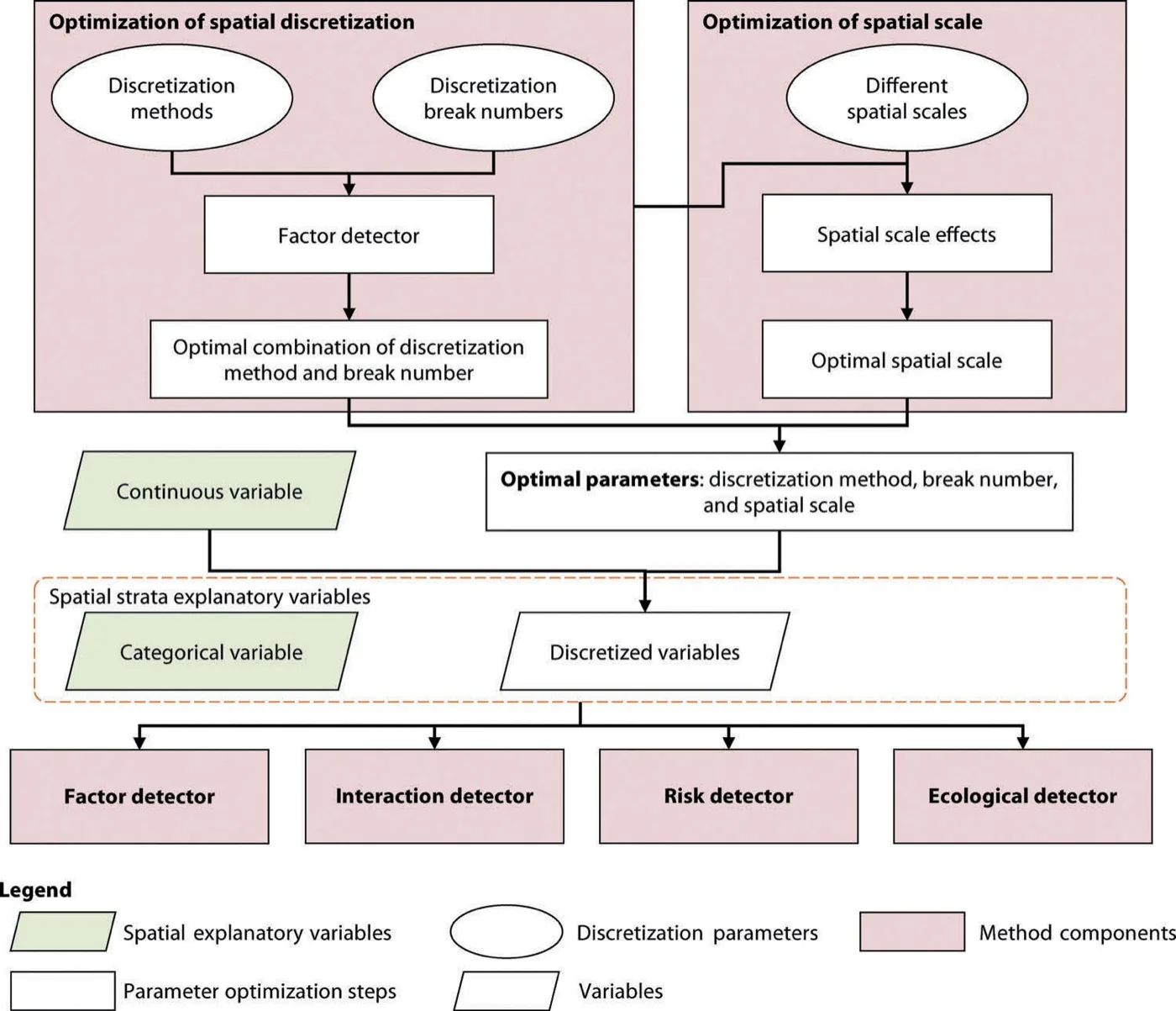
The four detectors

Detector	Question	Result
Factor	How much of the spatial variation of y does each factor explain?	q and its p value, per factor
Interaction	Do two factors together explain more than each alone?	q of the two factors overlaid, and the type of interaction
Risk	In which strata of a factor is y high or low, and do the strata differ?	Mean of y per stratum with its 95% interval; a t test for each pair of strata
Ecological	Does one factor explain significantly more than another?	Y or N for each pair of factors

When to use it

You want to rank candidate drivers of a spatial variable without assuming a linear relation: q only asks whether y differs between strata.
Your factors mix numbers and categories.
You want to know where y is high or low along each factor (the risk detector), which is often the finding readers remember.

Where it has been used

Field	Response y	Spatial unit	Study
Vegetation change	Change of NDVI	Grid cell	Song et al. (2020)
Road infrastructure	Pavement deflection and damage	1 km road segment	Song et al. (2018)
Public health	Incidence of H1N1 flu	Region	Example data of the R package GD

Any table of spatial units with one numeric response and a mix of continuous and categorical factors fits.

Bubble matrix of the interaction detector for 23 variables of road pavement deformation — **A published result.** The interaction detector in a study of road pavement deformation with 23 variables. Each bubble is a pair of variables and its size is the q of the pair. Source: Song et al. (2018), Fig. 8.

Keep in mindq measures association between the pattern of a factor and the pattern of y. It does not give the direction of an effect and does not show causation. The direction comes from the risk means.

2In Heterra

2.1 Prepare your data

One layer (points, polygons or grid cells) or one table. Each row is a spatial unit. The file can be a shapefile, GeoPackage, GeoJSON or CSV (Part 1 shows how to add data).

Field	Type	In the example
Response y	Number	`NDVIchange`
Continuous factors	Numbers, to be discretized	`Tempchange`, `Precip`, `GDP`, `Popdensity`
Categorical factors	Text classes or integer codes	`Climzone`, `Mining`
Boundary (optional)	A polygon layer	`opgd_boundary`: the outline drawn on the maps in the charts. It changes no result.

At least one factor of either kind is needed. The example has 713 simulated cells, so its numbers illustrate the tool and do not describe a real study.

2.2 Run the example, step by step

Open the tool from the Toolbox (Spatial heterogeneity → OPGD), click Tutorial, then Load Example. The cells and the boundary appear on the map, and the panel on the right is filled in for you.

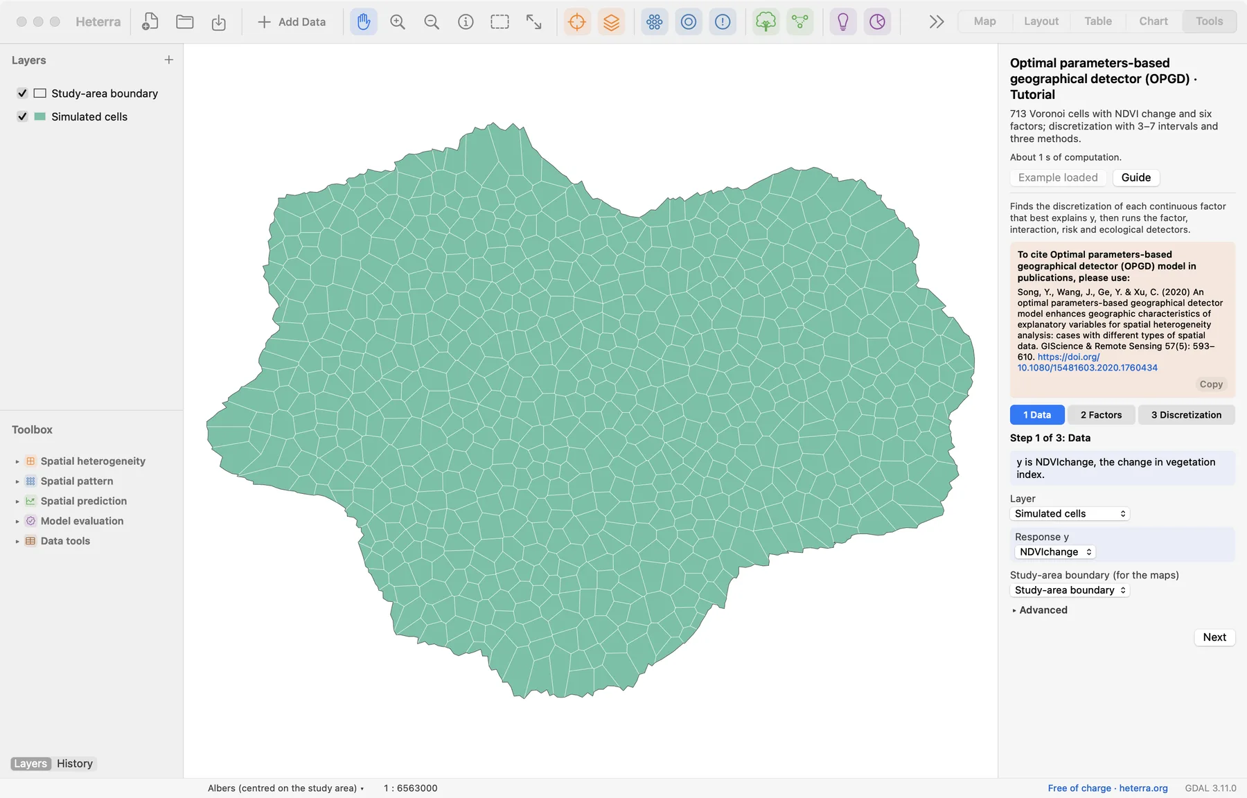
Heterra after Load Example: the 713 cells on the map and the OPGD panel at step 1 — After **Load Example**: the layers on the left, the map in the middle, the OPGD panel on the right at step 1 of 3.

The panel has three steps. Next moves on; Run appears at the last step, because only that step computes.

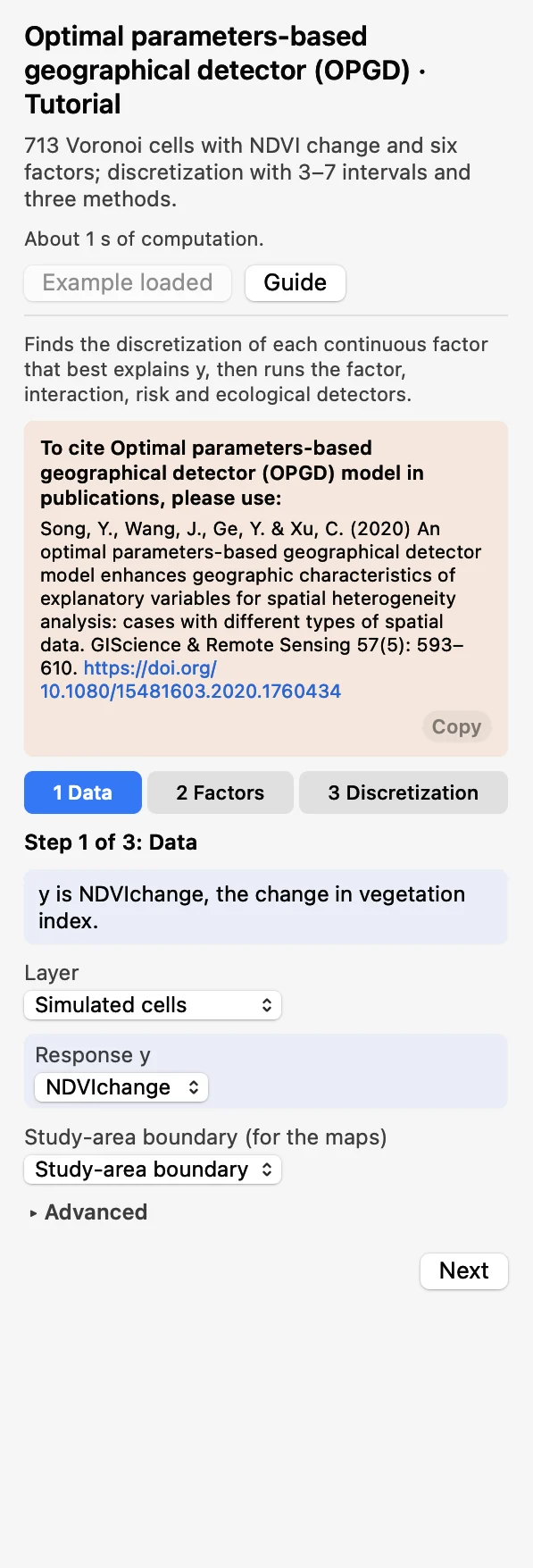DataChoose the layer and the Response y: NDVIchange. The boundary is optional.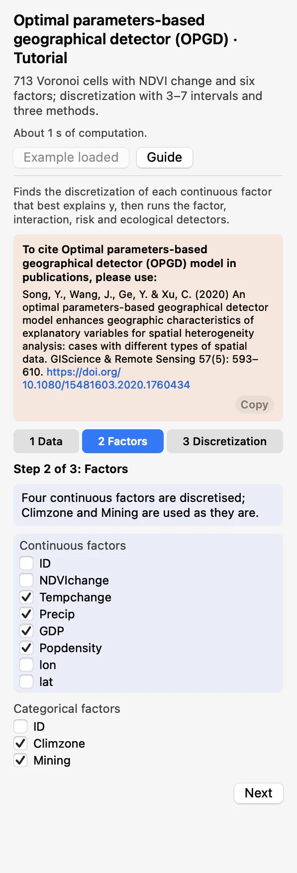
FactorsTick the continuous factors (to be discretized) and the categorical factors (used as they are).
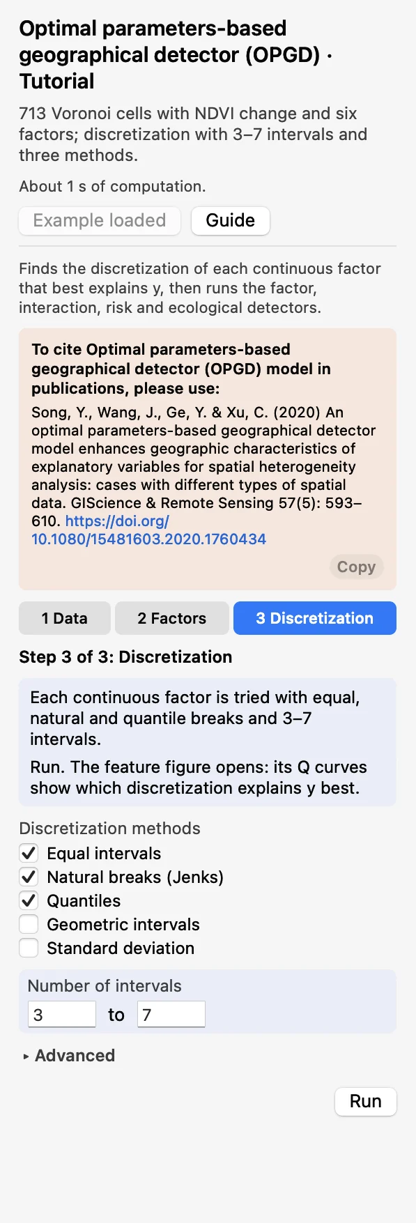DiscretizationKeep equal, natural and quantile breaks and 3 to 7 intervals. Click Run.

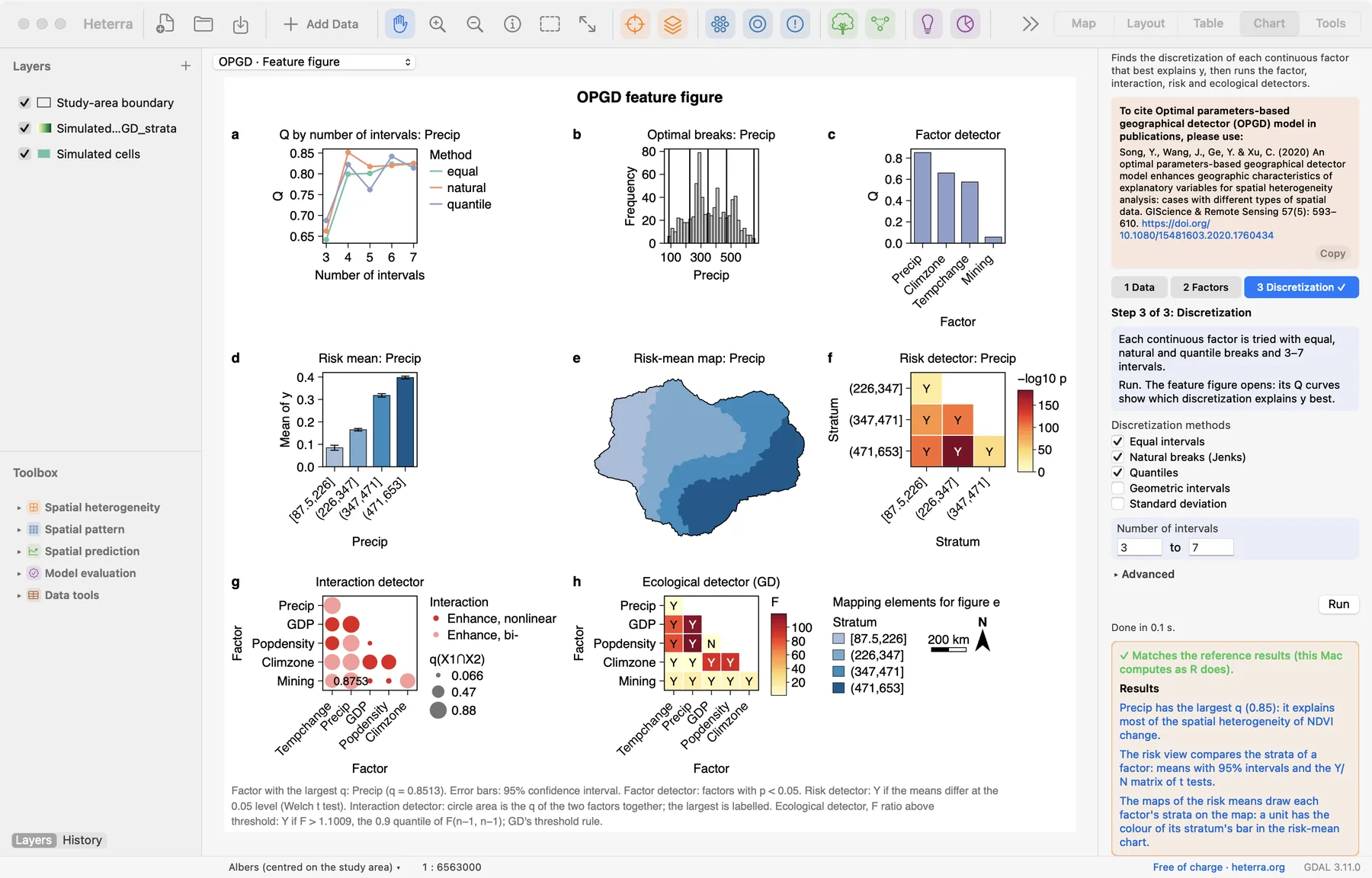
The run takes well under a second. The Chart page opens with the feature figure, and the panel lists every result under Outputs: tables first, then figures. A green line says that the results match the reference results computed with R.

Heterra after the OPGD run: the feature figure on the Chart page and the results in the panel — After **Run**: the feature figure. The menu above the figure and the Outputs list in the panel open the other figures and the tables.

2.3 With your own data

Add your layer (Add Data), open OPGD from the Toolbox and choose the layer in step 1.
Decide for each factor whether it is continuous or categorical. An integer code such as a soil class is categorical, even though it is a number.
Start with the default discretization (equal, natural and quantile breaks, 3 to 7 intervals). With more than about 20,000 rows, untick natural breaks, which are slow at that size.

Rows with a missing value in y or in any chosen factor are left out. At least 30 complete rows are needed.
A categorical factor needs at least two categories. Text categories are ordered alphabetically, numeric codes numerically.
A method and number of intervals that cannot be computed for a factor is skipped with a warning. The run stops only if nothing works for a factor.
Column names and category values are best written with English letters, digits and underscores.

3Reading the results

Read the results in this order: the discretization first (is it sensible?), then the factor detector (what matters?), then the risk detector (in which direction?), and last the interaction and ecological detectors (how do the factors compare and combine?).

3.1 Optimal discretization

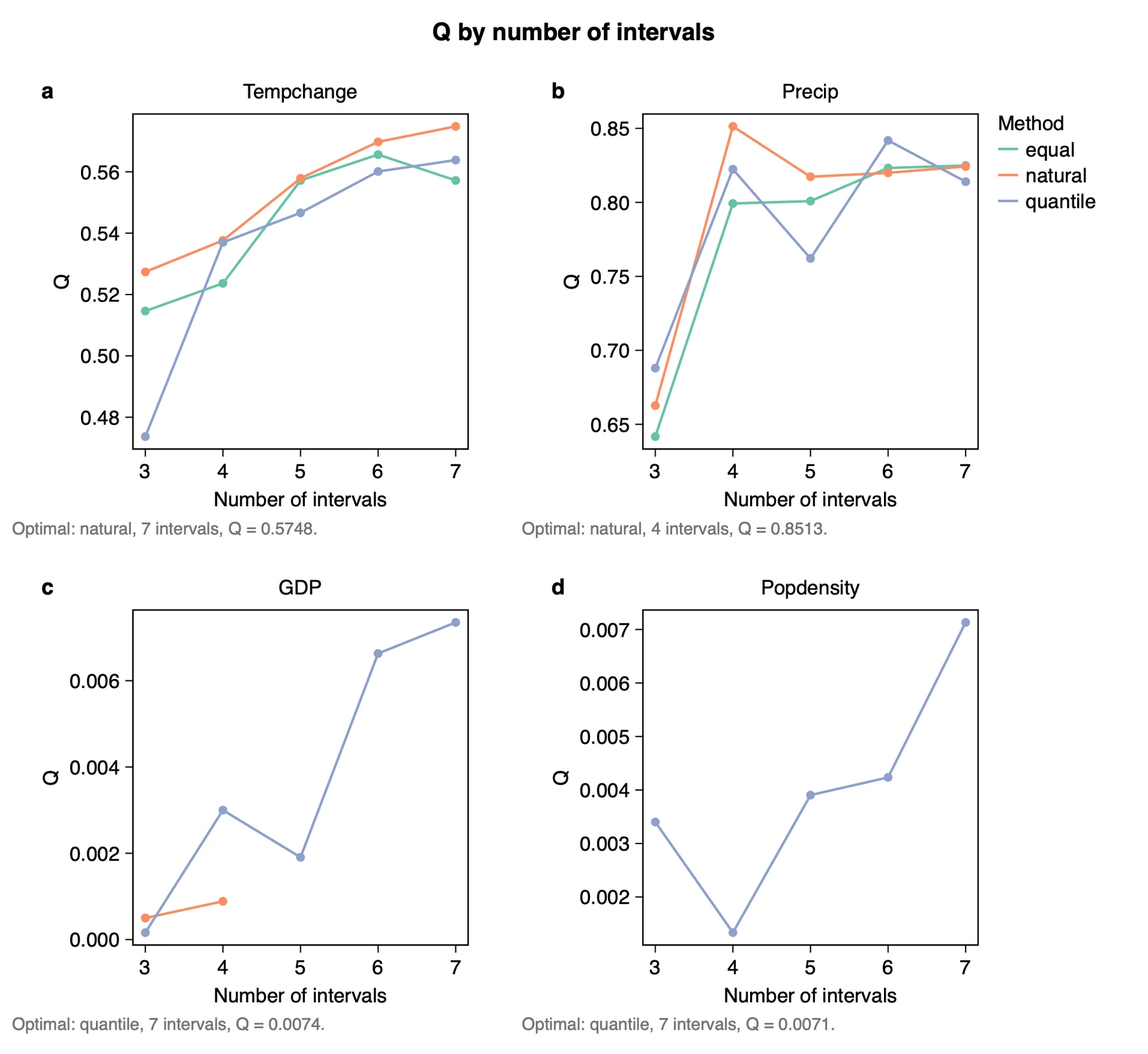
Q by number of intervals for Tempchange, Precip, GDP and Popdensity, one line per discretization method — **Q by number of intervals**, one panel per continuous factor. Each line is a discretization method; the optimal combination is written under each panel.

What it shows. q for every method and number of intervals that was tried. The combination with the largest q is kept. The table Optimal discretization lists it for each factor:

Factor	Method	Intervals	q
Tempchange	natural	7	0.575
Precip	natural	4	0.851
GDP	quantile	7	0.007
Popdensity	quantile	7	0.007

How to read it. q usually rises with the number of intervals, so look at the shape of the curve as well as its top. For Precip, q jumps from about 0.66 at 3 intervals to 0.85 at 4 and then stays near 0.82: four intervals are enough. When the largest q sits at the upper limit you set (7 here, as for Tempchange), the limit decided the answer; try a wider range to see whether q keeps rising or levels off.

The figure Optimal breaks draws the chosen breaks on the histogram of each factor, and the run adds fields named <factor>_strata to a copy of the layer, so that the strata can be mapped.

In a paper

"Continuous factors were discretized with the optimal parameters-based geographical detector (Song et al. 2020): equal, natural and quantile breaks with 3 to 7 intervals were compared, and the combination with the largest q was used for each factor (Table X)."

3.2 Factor detector

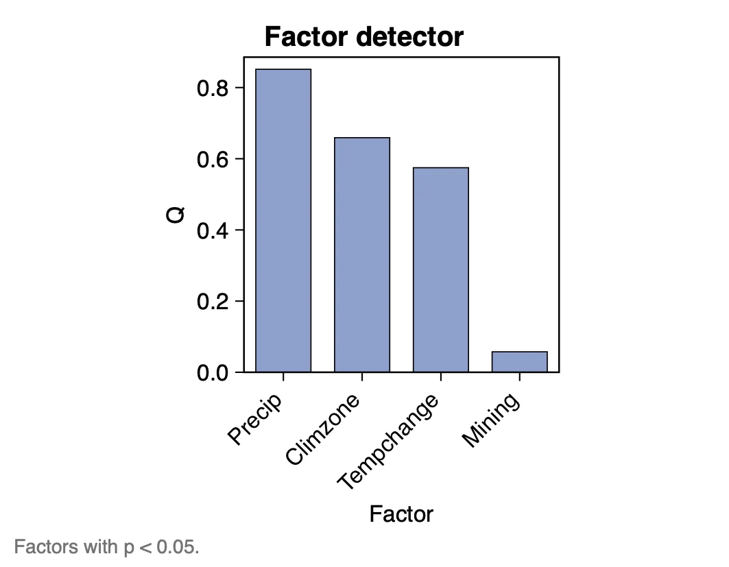
Bar chart of q for the factors with p below 0.05: Precip, Climzone, Tempchange, Mining — **Factor detector**: q of the factors with p < 0.05, largest first.

Factor	q	p
Precip	0.851	< 0.001
Climzone	0.659	< 0.001
Tempchange	0.575	< 0.001
Mining	0.057	< 0.001
GDP	0.007	0.79
Popdensity	0.007	0.69

How to read it. q is the factor's explanatory power: Precip explains 85% of the spatial variance of NDVI change, GDP less than 1%. Analyse q first. The p value says whether q differs from zero under the chosen discretization; with many units a small q can still be significant (Mining: q = 0.06, p < 0.001), so report both and judge importance by q.

In a paper

"Precipitation has the largest q (0.85): it explains the largest share of the spatial pattern of NDVI change, followed by climate zone (0.66) and temperature change (0.57). GDP and population density are not significant at the 0.05 level."

3.3 Risk detector

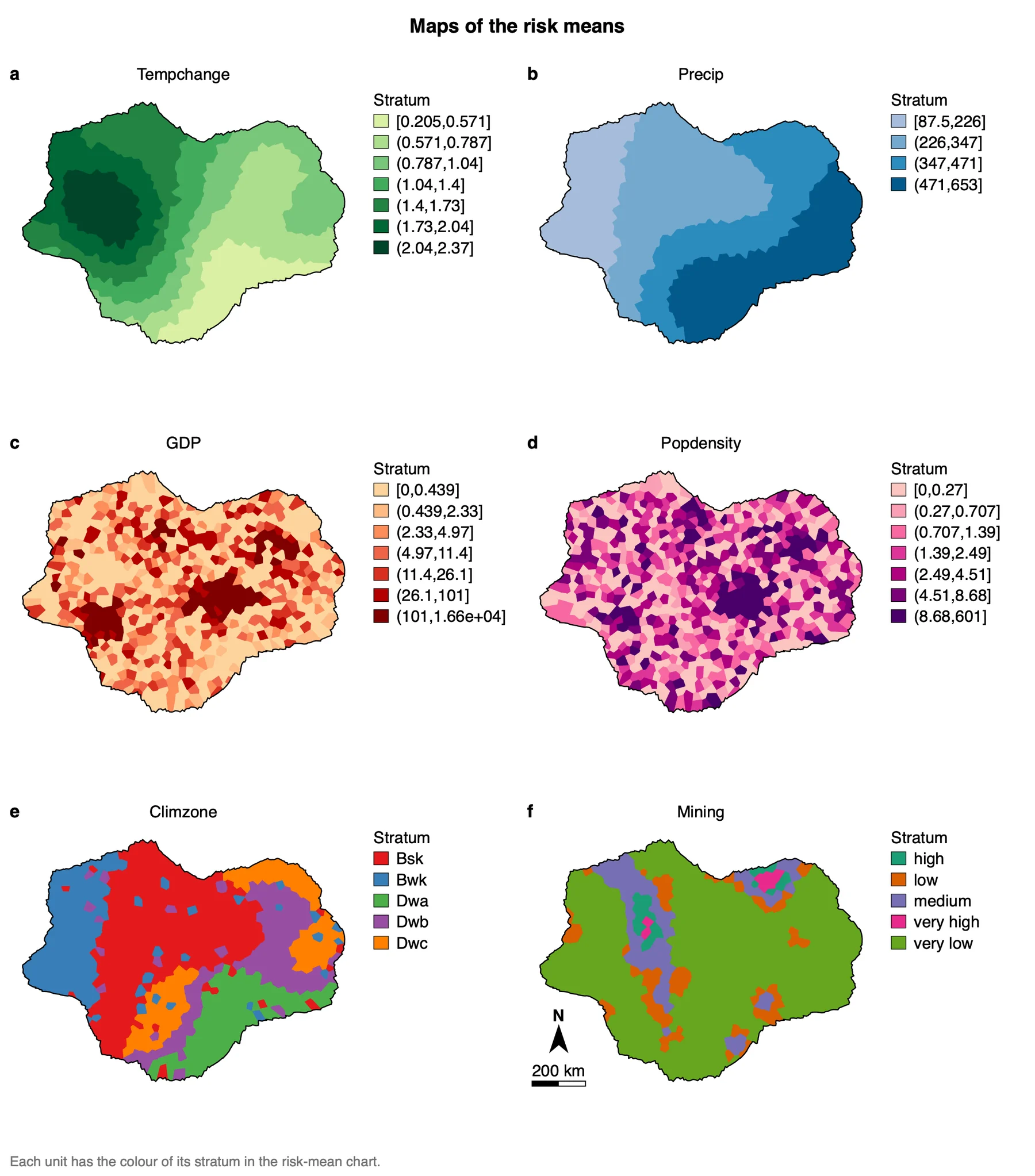
Maps of the risk means: one map per factor, each unit in the colour of its stratum — **Maps of the risk means**: one map per factor. Each unit has the colour of its stratum's bar in the risk-mean chart.

What it shows. The Risk means charts give the mean of y in each stratum with its 95% confidence interval; the maps show where those strata lie. For Precip:

Stratum of Precip	Units	Mean NDVI change	95% interval
[87.5, 226]	115	0.085	0.073 to 0.096
(226, 347]	244	0.165	0.160 to 0.171
(347, 471]	177	0.318	0.310 to 0.326
(471, 653]	177	0.398	0.391 to 0.404

How to read it. This is where the direction appears: NDVI change rises steadily with precipitation. The Risk detector chart is a matrix of Welch t tests between strata: Y means that the two strata's means differ at the 0.05 level. A row of N between neighbouring strata suggests that those intervals could be merged.

In a paper

"Mean NDVI change increases across the four precipitation strata, from 0.09 where precipitation is below 226 to 0.40 where it is above 471, and all pairs of strata differ significantly (Welch t test, p < 0.05)."

3.4 Interaction detector

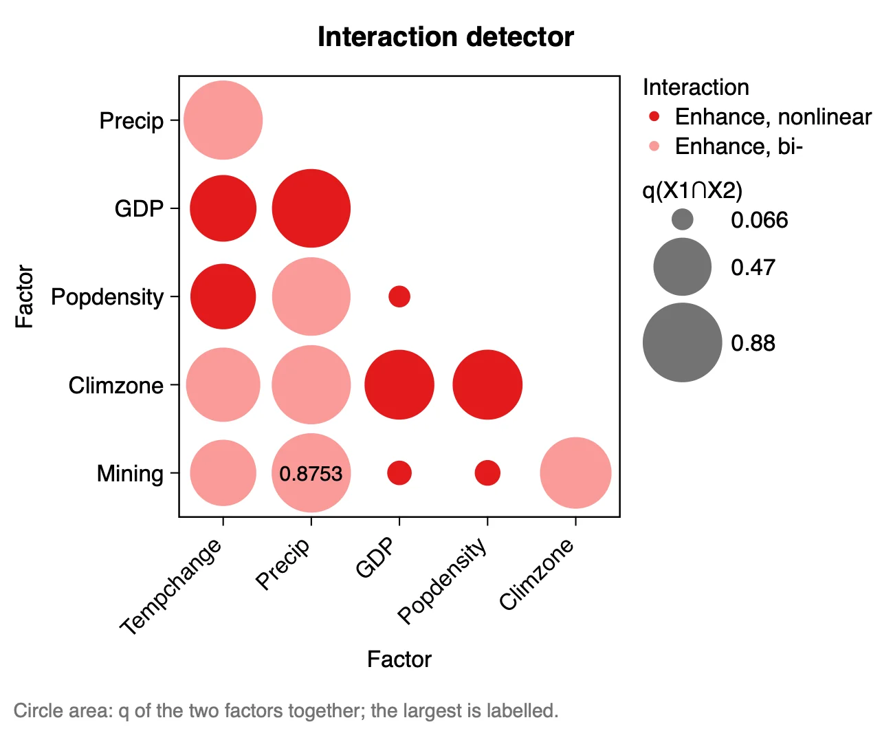
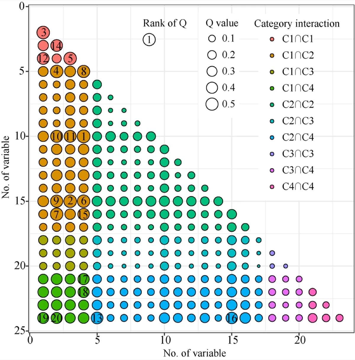
Interaction detector: circles sized by the q of two factors together, coloured by the type of interaction — **Interaction detector**: circle area is the q of the two factors together; the colour is the type of interaction.

What it shows. The two factors' strata are overlaid and q is computed for the combined strata, q(X1∩X2). It is compared with the two single values:

Type	Condition
Weaken, nonlinear	q(X1∩X2) < min(q1, q2)
Weaken, uni-	min(q1, q2) < q(X1∩X2) < max(q1, q2)
Enhance, bi-	max(q1, q2) < q(X1∩X2) < q1 + q2
Independent	q(X1∩X2) = q1 + q2
Enhance, nonlinear	q(X1∩X2) > q1 + q2

How to read it. Always read an interaction together with the two factors' own q. The largest value here is Precip ∩ Mining (0.875), but Precip alone already reaches 0.851: Mining adds little. A pair of weak factors can be "Enhance, nonlinear" and still explain almost nothing (GDP ∩ Popdensity: 0.066).

In a paper

"The strongest interaction is precipitation ∩ mining (q = 0.88, bi-factor enhancement), only slightly above precipitation alone (0.85). Every pair of factors enhances each other; none is independent or weakening."

3.5 Ecological detector

What it shows. For each pair of factors, whether one explains significantly more than the other. The table gives two definitions in use: the GD package's (Y or N: Y when the ratio of the two values reaches the threshold of the F distribution, 1.10 with 713 units) and the gdverse package's (F, p, Yes or No). They often disagree, so say which one you report.

How to read it. Use it to support a ranking: "Precip explains more than Tempchange" is backed by Y in that cell. GDP against Popdensity is N: their q values (both 0.007) cannot be told apart.

3.6 The feature figure

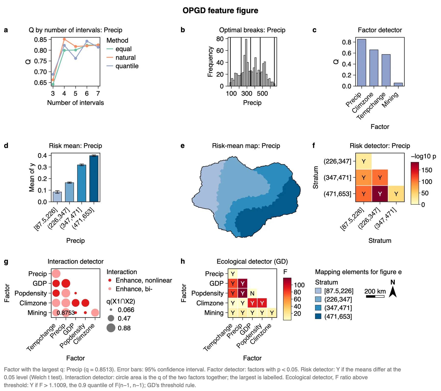
OPGD feature figure with eight panels — **Feature figure**: a, Q curves; b, optimal breaks; c, factor detector; d, risk means; e, risk-mean map; f, risk detector; g, interaction detector; h, ecological detector. Panels a, b, d, e and f are for the factor with the largest q.

The feature figure puts the main results on one page and is made for a paper's results section. Export it from the Chart page as PDF or SVG (vector) or PNG at 300 dpi; Data CSV saves the numbers behind it. Export results in the panel writes a report of the run with the method, the steps, the figures and the tables (Part 1).

3.7 Reading the results together

The detectors tell one story from four sides: which factors matter (factor detector), with which other factors (interaction detector), where y is high or low (risk detector) and how surely one factor outranks another (ecological detector). Read them in this order:

Optimal discretization: check that every continuous factor has a clear best combination.
Factor detector: the ranking and its significance.
Ecological detector: which gaps in the ranking are real.
Interaction and risk detectors: the pairs and the strata that carry the story. A factor with a small q of its own can still matter through an interaction.

What OPGD is notIt is not a prediction model: it gives no coefficients and no predicted values. It measures how much of the spatial pattern of y the strata of a factor explain. For a map of predicted values, use a method of Part 4.

3.8 From the results to a manuscript

Section	What to write	From Heterra
Methods	The q statistic; the discretization methods and the numbers of intervals compared; the four detectors	The settings of the run (in the exported report); table Optimal discretization
Results	Follow the order of the analysis: discretization, ranking of the factors, interactions, risk strata, significance of the differences. One finding per subsection, each with its q	Figure Feature figure or the single figures; tables Factor detector and Interaction detector
Discussion	Which factors lead together and which differ; the mechanism behind the strongest interaction; whether the ranking holds at another unit size	Table Ecological detector; a second run on coarser or finer units

Common pitfalls

Do not compare q values obtained with different search settings: more intervals explain more variance by construction. Fix the methods and the range of intervals, and let OPGD choose inside them.
Every stratum needs enough units. With a small sample, lower the largest number of intervals.
A large q is an association of patterns, not a cause, and has no direction.

4Exercises

Exercises 1 to 3 use the example. Exercise 4 is for your own data.

Exercise 1Read

Run the example with its settings. Which factor has the second-largest q, and is it continuous or categorical? Which two strata of Climzone have the lowest and the highest mean NDVI change?

Answer

Climzone (q = 0.659), a categorical factor. In the Risk means table, Bwk has the lowest mean (0.108) and Dwc the highest (0.379).

Exercise 2Change a setting

In step 3, tick only Equal intervals and run again. What are the optimal number of intervals and q of Precip now? What does the difference from the first run tell you?

Answer

With equal intervals only, the largest q of Precip is 0.825 at 7 intervals, against 0.851 with natural breaks at 4 intervals. A better method reaches a higher q with fewer strata: comparing methods is the point of OPGD. Both runs stay in History, so you can open either.

Exercise 3Interpret

A colleague writes: "GDP and population density interact strongly (nonlinear enhancement), so their joint effect on NDVI change is important." Check this against the interaction table. Is the sentence justified?

Answer

No. The type is "Enhance, nonlinear" because 0.066 is larger than 0.007 + 0.007, but the two factors together still explain under 7% of the variance. The type describes how q combines, not how large it is.

Exercise 4Your data

Run OPGD on your own layer with at least three factors. Write three sentences for a results section: one on the ranking of the factors (q and p), one on the direction of the strongest factor (risk means), and one on the strongest interaction compared with its two factors alone. Export the feature figure as PDF.

Checklist

Does each sentence give a number? Did you check that the optimal number of intervals is not simply the upper limit you set? Did you say which ecological-detector definition you used, if you report it?

References

Song, Y., Wang, J., Ge, Y. & Xu, C. (2020). An optimal parameters-based geographical detector model enhances geographic characteristics of explanatory variables for spatial heterogeneity analysis: cases with different types of spatial data. GIScience & Remote Sensing 57(5): 593–610. doi:10.1080/15481603.2020.1760434
Song, Y., Wright, G., Wu, P. et al. (2018). Segment-based spatial analysis for assessing road infrastructure performance using monitoring observations and remote sensing data. Remote Sensing 10(11): 1696. doi:10.3390/rs10111696
Wang, J.-F. et al. (2010). Geographical detectors-based health risk assessment and its application in the neural tube defects study of the Heshun Region, China. International Journal of Geographical Information Science 24(1): 107–127.
R package GD: cran.r-project.org/package=GD. Heterra's results match GD 10.9.